
Underdamped Simple Harmonic Motion
 المؤلف:
Papoulis, A
المؤلف:
Papoulis, A
 المصدر:
Probability, Random Variables, and Stochastic Processes, 2nd ed. New York: McGraw-Hill
المصدر:
Probability, Random Variables, and Stochastic Processes, 2nd ed. New York: McGraw-Hill
 الجزء والصفحة:
...
الجزء والصفحة:
...
 5-7-2018
 1409
1409
Underdamped Simple Harmonic Motion

Underdamped simple harmonic motion is a special case of damped simple harmonic motion
 |
(1)
|
in which
 |
(2)
|
Since we have
 |
(3)
|
it follows that the quantity
is positive. Plugging in the trial solution  to the differential equation then gives solutions that satisfy
 |
(6)
|
i.e., the solutions are of the form
 |
(7)
|
Using the Euler formula
 |
(8)
|
this can be rewritten
![x=e^(-(beta/2)t)[cos(gammat)+/-isin(gammat)].](http://mathworld.wolfram.com/images/equations/UnderdampedSimpleHarmonicMotion/NumberedEquation7.gif) |
(9)
|
We are interested in the real solutions. Since we are dealing here with a linear homogeneous ODE, linear sums of linearly independent solutions are also solutions. Since we have a sum of such solutions in (9), it follows that the imaginary and real parts separately satisfy the ODE and are therefore the solutions we seek. The constant in front of the sine term is arbitrary, so we can identify the solutions as
so the general solution is
![x=e^(-(beta/2)t)[Acos(gammat)+Bsin(gammat)].](http://mathworld.wolfram.com/images/equations/UnderdampedSimpleHarmonicMotion/NumberedEquation8.gif) |
(12)
|
The initial values are
so  and
and  can be expressed in terms of the initial conditions by
The above plot shows an underdamped simple harmonic oscillator with  ,
,  for a variety of initial conditions
  .
.
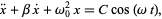
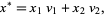
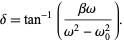
For a cosinusoidally forced underdamped oscillator with forcing function  , so
, so
 |
(17)
|
define
for convenience, and then note that
We can now use variation of parameters to obtain the particular solution as
 |
(24)
|
where
and the Wronskian is
These can be integrated directly to give
Therefore,
where use has been made of the harmonic addition theorem and
 |
(33)
|
REFERENCES:
Papoulis, A. Probability, Random Variables, and Stochastic Processes, 2nd ed. New York: McGraw-Hill, pp. 525-527, 1984.
 الاكثر قراءة في معادلات تفاضلية
 اخر الاخبار
اخبار العتبة العباسية المقدسة


